Slouching toward Pandas

Using LET and LAMBDA to raise the spreadsheet skill ceiling

Why use spreadsheets for newsroom data? They may have been our best option in the Lotus 1-2-3 days, but in 2023 data journalists have many more choices. Notebook tools like Jupyter or Observable offer expressive syntax that can fall back to a real programming language, they’re visually appealing, and they’re often extremely powerful. As a result, they’re now the default for many teams.

Spreadsheets have not historically had most of these advantages, but they do have an almost-subterranean skill floor. I hate to see a reporter manually add numbers from two cells together with a calculator and then type the result into a third cell. But they can do that if they want to contribute to my analysis, whereas most of them are never going to use a Pandas dataframe. If they want to learn to do some basic cell calculations, that’s not so hard. Google Sheets are also deeply collaborative and shareable in a way that most notebooks are not.

I think it’s reasonable to decide that the power of notebook-based tooling is worth the barrier to entry and loss of frictionless collaboration. But if you, like me, think those are valuable qualities in a default toolkit, then the question becomes: how do we raise the skill ceiling closer to (or even equivalent to) notebook tools, so that experienced data reporters don’t feel like they’re trapped in the bronze age while everyone else shows off the latest ironworks?

This isn’t an impractical goal. Unknown to a lot of people, after years of stagnation, spreadsheets have made huge jumps in capability, to the point that I think they can be almost as expressive as a notebook or even a query language like SQL. I’ve already written about how to use named ranges and array formulas to clarify lookups and filters. Now I’d like to talk about two new Lisp-inspired functions that can help close the gap between Sheets and other data tools: LET and LAMBDA.

LET the right one in

Of the two, LET is easier to understand. It’s basically a wrapper to assign a local name to a value, but only within the scope of the current cell. For example, here’s a cell that computes the post-tax price for an item:

=LET(
  price, .99,
  tax_rate, 0.07,
  price + (price * tax_rate))

In this case, we define two local variables, price and tax_rate, with the values .99 and .07, respectively. The final argument to LET is the calculation using those variables (the “return value” in other languages). You can start to see how this might make even simple formulas more self-documenting, but we can really start to see the benefits of LET if we need to use conditionals or other branching code.

Let’s say that we were computing school testing aggregates based on student data (a named range called student_scores), but we want to suppress any result that’s based on fewer than 10 individuals. Without LET, that formula would probably look like this:

=IF(COUNT(FILTER(student_scores, school = A2)) < 10, "-", AVERAGE(FILTER(student_scores, school = A2)))

In this formula, the filter clause is repeated in two places, once for the length test and again for the actual result. If our selection criteria gets more complicated (say, our sheet contains multiple test subjects and we only want one of them), we’ll have to update both filters in sync. Contrast this with a version that uses LET:

=LET(
  scores, FILTER(student_scores, school = A2),
  IF(COUNT(scores) < 10, "-", AVERAGE(scores)))

Now we only have to maintain our filter in one place, and there’s a lot less noise in the formula, since we can assign human-readable names to sections of it. Note the indentation: you can add newlines to your formulas in Sheets by pressing Ctrl-Enter (on Windows) or Command-Enter (on a Mac). I like to put each variable declaration on its own line in LET statements for greater legibility.

Leg of LAMBDA

While LET provides local variables, LAMBDA gives us the ability to compose functions for reuse. You can call a lambda function immediately, give it a local name using LET, or you can use the new “named function” panel to make them globally available to any cell in your sheet. LAMBDA expressions can also use other functions as inputs. For example, here’s a SUPPRESS function:

=LAMBDA(
  result_array, fn,
  IF(COUNT(result_array) < 10, "-", fn(result_array)))

Once this is assigned to a named function in my workbook, I can call this in a LET, passing in my scores and a lambda that says what to do with the unsuppressed results:

=LET(
  scores, FILTER(student_scores, school = A2),
  aggregate, LAMBDA(input, AVERAGE(input)),
  SUPPRESS(scores, aggregate))

I can change the aggregation by swapping out the lambda that I pass into SUPPRESS, such as asking for the standard deviation instead of the average:

=LET(
  scores, FILTER(student_scores, school = A2),
  aggregate, LAMBDA(input, STDEV(input)),
  SUPPRESS(scores, aggregate))

Sadly, although it would be nice to just pass in the aggregate function directly, built-in functions must be wrapped in a LAMBDA.

// this won't work
=SUPPRESS(E:E, SUM)

// wrapping SUM in a lambda creates a callable function
=SUPPRESS(E:E, LAMBDA(v, SUM(v))

It’s worth noting, if you’re curious, that LET is effectively “syntax sugar” over LAMBDA: you can get the same effect by creating a function and immediately calling it with values to fill its arguments. The following two formulas do the same thing, but the LET formulation is probably easier for most people to reason about, since the variable values are closer to their name declarations.

=LAMBDA(x, y, x + y)(1, 2)

=LET(x, 1, y, 2, x + y)

LAMBDA in turn seems to be sugar over ARRAYFORMULA, at least according to some of the error messages I’ve seen when working with it. For that reason, while testing, it’s often a good idea to develop a LAMBDA from a series of cell operations and then integrate them into a final form for your named function definition, just as you’d step-debug a complex procedure in a traditional language.

Case study #1: school transfer counts

One interesting thing about LET is that its binding expressions are cumulative–any variable definition can use the previous variables in its declaration. Even if you’re not using them in multiple places, you can make a very complex formula easier to understand by breaking down its component parts into named values and processing them line by line.

Here’s a real-world case: one of our bureaus had a spreadsheet containing individual student records from two points in time: where they were enrolled a number of years ago, their grade level at the time, and where they were enrolled more recently (assuming they were still enrolled).

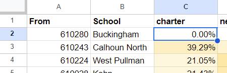
I wanted to find the percentage of students ten years ago at a given school ($A2, the row prefix) had ended up at a specific type of school now (C$1, the column header). The result is basically a pivot, but the cell values are computed based on two input sets—the number that are still enrolled, and all students originally at a given school.

The formula uses two named functions set up in the workbook for convenience sake: the MATCHGRADES named function only finds students in grades PE-2, and COUNTFILTERED correctly handles counting non-numeric values (COUNTA(FILTER(x)) will return 1 for no matches, since it counts the error as a value). The definitions for those look like this:

// MATCHGRADES
=MATCH(grade, { "PE", "PK", "K", "1", "2" }, 0)

// COUNTFILTERED
=IF(ISERROR(filtered), 0, COUNTA(filtered))

Here’s the final formula for cell C2, which I then dragged out to fill the complete table:

=LET(
  in_school, ARRAYFORMULA(students_from = $A2),
  in_grade, ARRAYFORMULA(MATCHGRADES(students_grade)),
  still_enrolled, ARRAYFORMULA(students_enrolled = TRUE),
  went_to, ARRAYFORMULA(students_to_type = C$1),
  enrolled, FILTER(students_id, in_school, in_grade, went_to, still_enrolled),
  all, FILTER(students_id, in_school, in_grade, still_enrolled),
COUNTFILTERED(enrolled) / MAX(COUNTFILTERED(all), 1))

Breaking this formula down to its component pieces, in_school, in_grade, still_enrolled, and went_to are all arrays containing true/false results for each student in the source data:

• in_school - did the student attend the school for this pivot row?
• in_grade - were they in the grades we want to look at?
• still_enrolled - are they still enrolled?
• went_to - did they end up at the school type in this pivot column (charter, neighborhood, alternative, etc.)?

From these arrays, we create two filtered lists of student IDs, one that matched on all conditions and one that matches on school, grade, and enrollment (but for any school type). With those two filtered sets, the last line computes the final percentage of students who went to a given school, in the desired grades, and are still enrolled at a school of a given type.

Without LET, I’d probably have needed a column in each row for the total enrolled students at each origin school, then columns for the counts of enrolled students in each category, then a duplicate set of columns that find the percentage from those figures. The result would be more explicit, but also a lot less compact. Each person will need to determine where the line is for that trade-off, but it’s exciting to have the options. On a team with some fluency in this technique, I don’t think this example is excessive.

Case study #2: Filling sparse columns

Perhaps knowing that if you wave something called LAMBDA in front of a bunch of nerds, they’re going to expect that you give them functional programming tools, Sheets does include some higher-order functions now like MAP and REDUCE. Most of the time, these are not terribly useful, since we already have first-class support for ARRAYFORMULA and a handy set of aggregate functions available to us, but it’s good to have them around just in case.

However, one unambiguously helpful lambda-dependent function is SCAN, which generates a sequence of values for each cell in a range based on both its value and the previous output–it’s like a REDUCE that shows its work. You can use this for a number of cool tricks, but the most common is to fill in sparse columns.

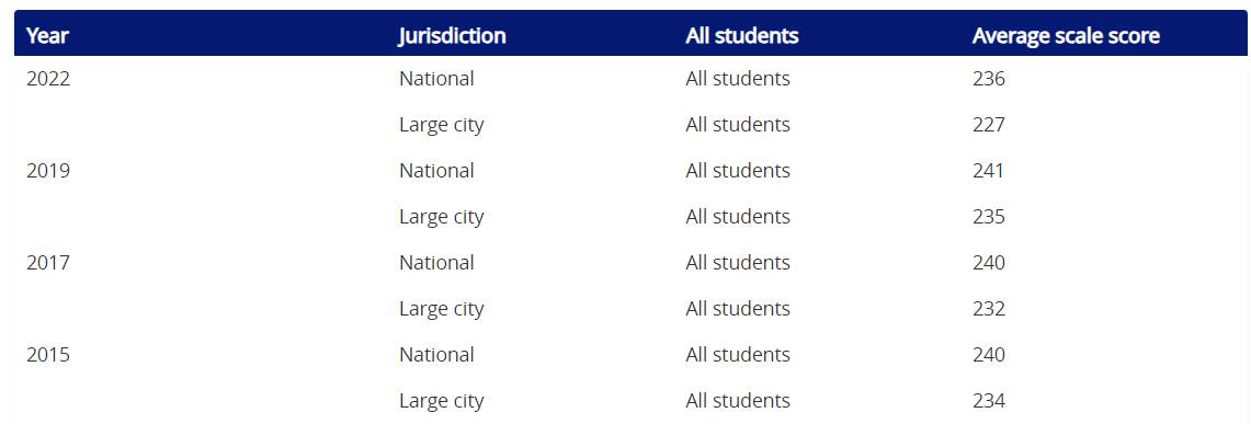
Take, for example, the NAEP test results over time. If you run this query in the data explorer, you’ll get a table with individual rows for national and city results for each year–but only the first row will have the year displayed:

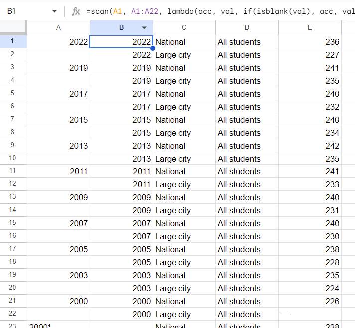
When you copy and paste this into a sheet for visualization, you’ll want to fill in the missing year values, but clicking on each one to fill down is almost as tiresome as adding the values by hand. It’s possible to write an IF that will fill in the values, but you’ll have to make sure that fills the entire column, which can be a problem if there are gaps on both sides. Instead, here’s SCAN to the rescue:

=SCAN(A1, A1:A22, LAMBDA(acc, val, IF(ISBLANK(val), acc, val)))

The SCAN function takes three arguments. The first is a starting value, which for our purposes is just the start of the range (2022). The second is the range we want to cover, which in this case is our sparse column (I’ve selected the rows corresponding from 2022 through 2000). Finally, we give it a lambda that receives the previous output (acc, for “accumulator”) and the current cell value. If the current value is blank, we repeat the last value. Otherwise, we replace it with the new year.

It used to be that if I didn’t want to do this kind of data cleanup by hand, I’d have to switch over to the Apps Script editor and write some extension code, then add a note for other team members in case they needed to recreate the results. Now, everything is right there in the sheet, and I don’t need to context switch or remember the SpreadsheetApp API.

Essentially, LET and LAMBDA don’t just make our formulas more readable: they also create options for extensibility that would have previously required leaving the workbook for another tool.