She has the range
Superior spreadsheet lookups with arrays, named ranges, and filters
There’s a reason that VLOOKUP is often seen by reporters and data newcomers as the standard of “spreadsheet wizardry.” It’s hard to teach and hard to learn – a relic of a grimly cryptic era in software design. If you’re using the newest version of Office, you can (and probably should) use Microsoft’s new XLOOKUP. But for those of us using Google Sheets to collaborate (or who have been carting a copy of Office 2007 around for 15 years), is there a way to make table lookups feel less like we’re bobbing for apples in a piranha tank?
After spending a year trying to tame the workbooks behind NPR’s COVID graphics, and then falling headlong into Chalkbeat’s education data analysis, I think the answer is yes. Even better, the techniques we’ll use to supercharge VLOOKUP can level up almost any spreadsheet formula.
VLOOKUP the hard way
A typical VLOOKUP formula usually appears something like this:
=VLOOKUP(A2, second_sheet!C2:H, 5, false)
To break that down:
A2is the ID that we’re using to find a given row.second_sheet!C2:His the range of cells that we’re going to search, looking for the value in A2 in the first column of the range (in this case, column C).5means that we want to get the value from the fifth column in the row that matches A2, which is… (counts up from C on my fingers) column G.falsemeans that the VLOOKUP must match the value exactly, as opposed to finding the “closest” match.
This packs a lot of potential points of failure into a small bit of code. There’s only one search value, so you can’t match something across multiple columns (say, state and year). Your search table has to always be set up so that the keys are physically to the left of the desired value, which isn’t always possible. You have to be able to count the columns in a piece of software that normally refers to them by letter. And if you forget that last parameter, VLOOKUP will happily hand you a random value instead of matching your search or erroring out.
Luckily, Google Sheets offers us some ways that we can turn VLOOKUP into something close to XLOOKUP (and in some cases, better), by leaning into three of its array-oriented language features.
Simplifying search with named ranges
We can use named ranges in Google Sheets to give a nickname to a group of cells for use in formulas – effectively, a variable name. This becomes incredibly useful anytime that you need to work across multiple sheets in a workbook. I almost always create them for columns in a table that I’ll need elsewhere. For example, let’s say we’re writing a report where we want to find the number of schools in a column that are above 50% in COVID test rates:
=COUNTIF('school testing rates'!G:G, ">.5")
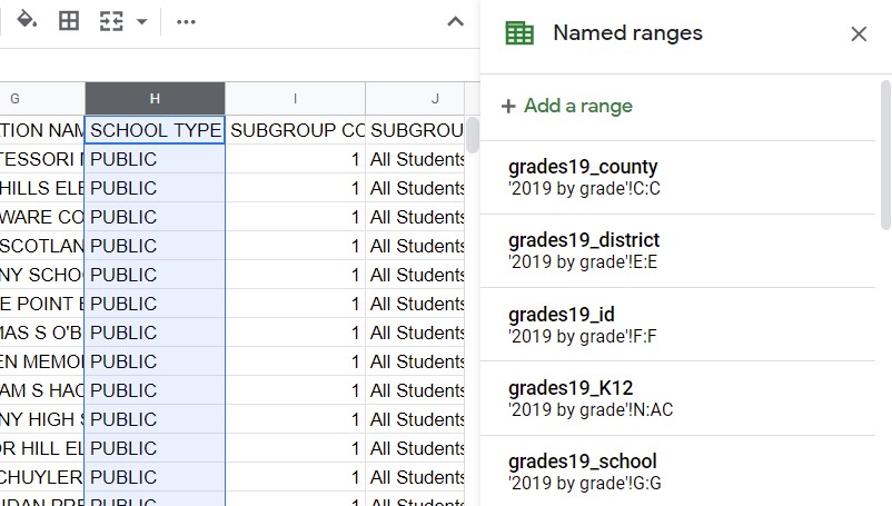
To write this out manually, I always end up having to switch between workbook tabs repeatedly to make sure I’ve got the right column, and if I give my sheets descriptive names with spaces they become increasingly painful to reference in formulas. Whereas if I create a named range, I can reference it easily no matter what the sheet is named, and Sheets will even autocomplete it in formulas for me. So in this case, I click on the column header for the column containing the test values, go to the Data -> Named Ranges menu, and then call it schools_testing. The resulting reference can then replace the sheet coordinates in the formula:
=COUNTIF(schools_testing, ">.5")
It’s much easier to write, and also much easier for newcomers to the sheet (meaning either my team or myself in two weeks) to figure out what that formula is doing.
Since we’re replacing the actual sheet name in the formula, it’s useful to have a reliable scheme for named ranges so that they’re easy to identify. I usually try to stick with a variation on sheet_column, so that it’s easy to identify named ranges from the same table. For example, in a New York attendance story, I created ranges for the per-grade statistics by year that were grades19_group, grades19_total, grades19_county, and so on.
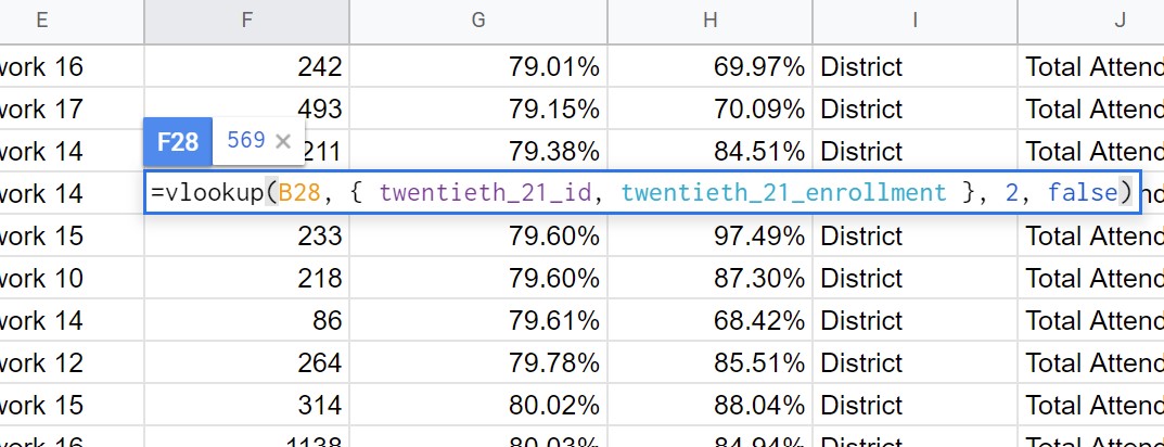
In the context of a VLOOKUP, we can combine named ranges with Google Sheets arrays to make self-documenting search formulas without ever having to count our columns or have a specific table arrangement. Here’s how it looks:
=VLOOKUP(A2, { school_ids, school_testing }, 2, false)
The { a, b, c } syntax in Sheets constructs an array from the named cells, which is kind of like a “virtual sheet,” with columns separated by commas and rows by semicolons. In the formula above, instead of directly referencing a range in the sheet, we define an array out of named ranges, with the first column being the school ID codes and the second being the value we want to get (testing rates).
Because we’re building this search table ourselves, it only needs two columns: one for the key and one for the value. That means we don’t need to count columns in our selected range anymore: the third parameter in the VLOOKUP formula will always be 2. And they can be in any order in the original sheet – VLOOKUP will only ever see our custom array, which we can reorder as we see fit. Flaunt convention! Put the keys at the end of the table! God is dead, and everything is permitted!
There’s a couple of things to watch out for with this technique. Your columns for your array need to be the same size, and they should start at the same row, or the lookup will be misaligned. For example, you can’t create an array as { column_a, column_b }, if column_a is defined as A2:A and column_b is B:B, because the dimensions will be different (B is one row taller).
Handling multi-column matches with filters
Sometimes you need to find a value based on matches across multiple columns, but neither XLOOKUP nor VLOOKUP handles that particularly well. For example, in many states, schools are identified by both a district and a school ID code, the latter of which is not guaranteed to be unique across districts. If you need to find a single school, you need both IDs, but the lookup functions can only match one value at a time.
The common solution for this problem is to create a third column in both your tables that combines the two IDs, and then perform the lookup based on that. This works, but it clutters the data and requires a new key column for each combination of lookup values. For example, if you also need to specify a year, you now need an additional key column for district & school & year.
Instead of altering our tables, we can use FILTER to winnow the possibilities that we feed to our VLOOKUP:
=VLOOKUP(A2,
  FILTER(
    { school_id, school_testing },
    school_district = B2,
    school_year = C2
  )
)
The FILTER function (which is only available in Sheets and the newest versions of Excel) takes in a set of values, followed by a list of condition arrays to control the filter. A row from the first argument will only be included in the output if the corresponding rows in all of the condition arrays are TRUE or its equivalent.
In our example, we’ve created an array of the school IDs and testing results, but then filtered that array by district and year before feeding it to VLOOKUP. As a result, the VLOOKUP can safely look for just the school ID, knowing that the other columns have already been restricted to a universe where that ID is unique.
You can also do all of this just through a filter:
=FILTER(
  school_testing,
  school_id = A2,
  school_district = B2,
  school_year = C2
)
However, if FILTER finds multiple results that match, it’ll happily overflow into multiple rows of the output, where VLOOKUP will only return the first one it finds. I think VLOOKUP is clearer in intention, but FILTER is useful for catching errors where your data might contain duplicate keys.
Even outside of VLOOKUP, named ranges make FILTER so much more expressive, it’s hard to go back to the days before I used them religiously. Take, for example, this formula I recently wrote to find the enrollment at NYC public schools across five counties:
// using explicit sheet references, like a fool
=SUM(
  FILTER(
    '2021 by grade'!K:Z,
    MATCH('2021 by grade'!C:C, analysis!G2:G6, 0),
    '2021 by grade'!H:H = "PUBLIC"
  )
)

// using named ranges, wisely
// grades21_* ranges always point to the "2021 by grade" sheet
=SUM(
  FILTER(
    grades21_k12,
    MATCH(grades21_county, nyc_counties, 0),
    grades21_type = "PUBLIC"
  )
)
The latter is much easier to read, and doesn’t require me to flip between multiple sheets to understand its conditions. The MATCH in particular is much clearer that it identifies rows with a county matching any entry in the nyc_counties range, instead of just showing two arbitrary sheet locations.
A unified theory of Sheets ranges
What is it that these techniques have in common? They involve a shift in our mental model of spreadsheet data: instead of thinking about it as a grid of cells in specific physical locations, we can start to think about it as lists of values that can be compared or matched against each other. I first started to make this conceptual leap when I watched a 2016 talk on functional Excel by Felienne Hermans.
From this perspective, formulas in Sheets are not dissimilar from list comprehensions in Python, functional array processing in JavaScript, or a SQL query:
// Sheets
=FILTER(school_names, school_testing > .5)
# Python
majority_testing = [ school.name for school in schools if school.testing > .5 ]
// JavaScript
var majorityTesting = schools.filter(s => s.testing > .5).map(s => s.name);
-- SQL
SELECT school_name
FROM schools
WHERE testing > .5;
Indeed, the closest comparison in computer science is an array-oriented language like APL, albeit without the cryptic keyboard symbols. Adding ARRAYFORMULA to our bag of tricks even allows us to perform arithmetic and use single-value formulas on an entire range of values in a very similar way to vector operations in those languages:
// add four to each item in the range and return 5 cells
=ARRAYFORMULA(A1:A5 + 4)

// create a new summary table of budget totals from individual spending columns
={ budget_item, ARRAYFORMULA(budget_salary + budget_equipment + budget_other) }

// quickly generate a header row of 12 months
=ARRAYFORMULA(date(2022, SEQUENCE(1, 12), 1))
Of course, spreadsheet formulas are unlikely to ever be as clear or expressive as a full-featured programming language, especially those (like SQL) that are designed explicitly for table manipulation. But using these techniques we can close the gap significantly, making Sheets much more readable and maintainable in the process.